

The OR Solver node solves optimization and constraint-satisfaction problems from within an automation. Define a mathematical model- variables, constraints, and an objective- and the node finds the best feasible solution using the solver type you choose.
Overview
Operations research (OR) solvers find optimal assignments, schedules, allocations, and routes when the solution space is too large for brute-force search. The OR Solver node exposes this capability without requiring code: you build the model step by step using the node's operations, then call Solve.
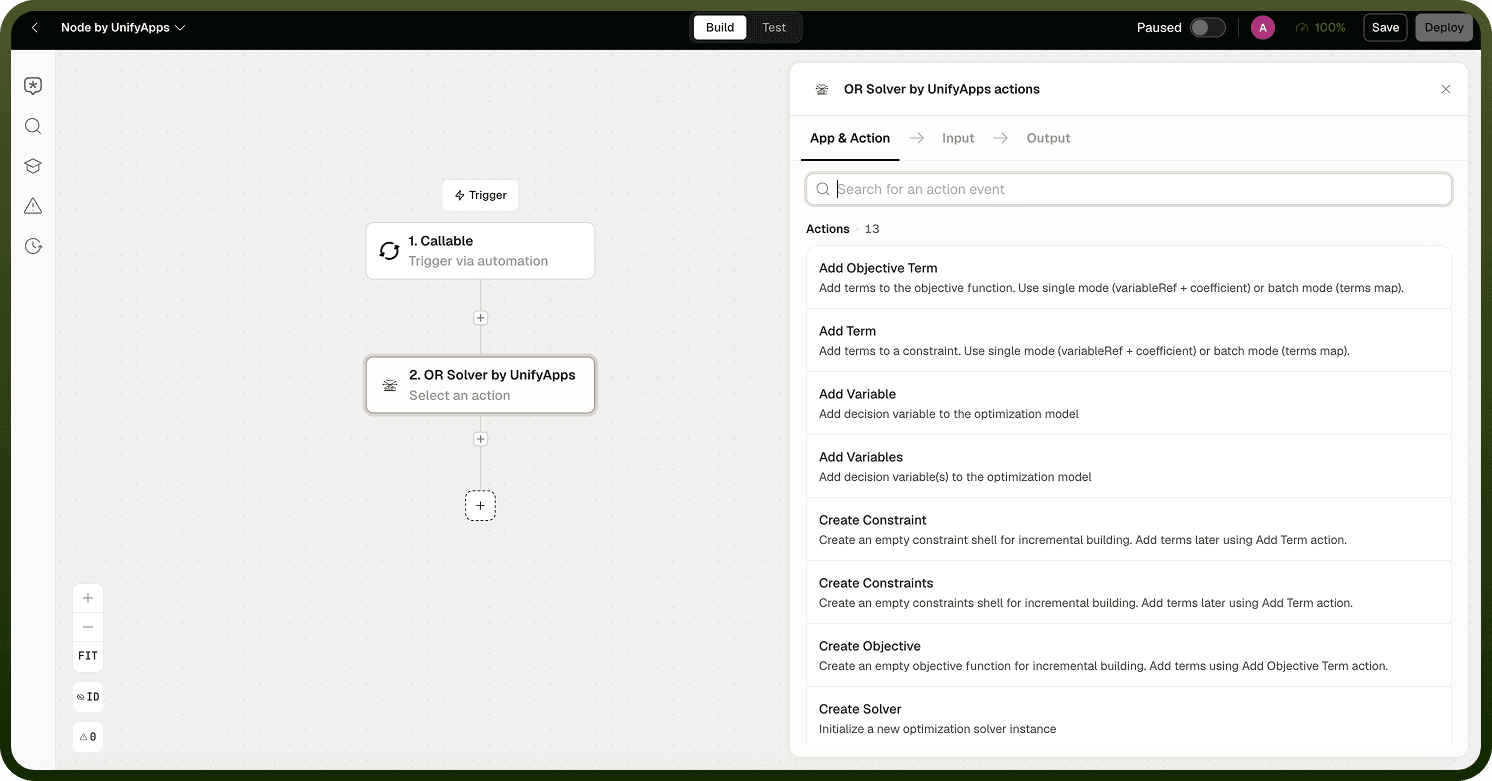
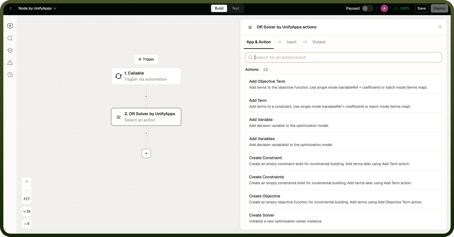
Building a Model
A model is built in sequence — each operation adds to the solver session you pass forward:
Create solver — initialize a solver session and choose the solver type. The solver reference is returned and passed to every subsequent operation.
Add variables — define the decision variables the solver may adjust. Each variable has a name, domain (continuous or integer), and bounds.
Add constraints — define the rules the solution must satisfy. Constraints reference the variables you declared and specify bounds or relationships between them.
Define objective — specify what to maximize or minimize, expressed as a linear combination of your variables.
Solve — run the solver. The output contains the solution status and, if feasible, the values of every variable.
Note: Always pass the solver reference from one operation to the next. Each step mutates the same session, so losing the reference mid-chain leaves the model incomplete.
Solver Types
Choose the solver type when you create the solver. The choice determines which class of problems the engine can handle:
GLOP — linear programming. Use when all variables are continuous and all constraints are linear. Fastest option for linear models.
SCIP — mixed-integer programming. Use when some variables must take integer values (e.g., whole units, binary on/off). More powerful than GLOP but slower.
CBC — another mixed-integer solver. Similar capability to SCIP; useful as an alternative if SCIP times out on a particular model shape.
CP-SAT — constraint programming and satisfiability. Use for combinatorial problems — scheduling, assignment, and routing — where you need to satisfy a set of hard constraints.
HiGHS — high-performance LP and MIP solver. Use for large-scale linear and mixed-integer models where performance is critical.
Time Limits and Async Execution
Complex models can take a long time to solve. Set a time limit on the Solve operation to cap how long the solver runs. When the limit is reached, the solver returns the best feasible solution found so far (which may not be globally optimal) rather than failing.
For large models, enable asynchronous execution — the automation pauses while the solver runs independently, then resumes with the result when it finishes. This avoids blocking the run for long-running solves.
Checking the Solution Status
The Solve operation returns a status field alongside the variable values. Always check this before using the result:
Optimal — the solver found the best possible solution.
Feasible — the solver found a solution that satisfies all constraints, but optimality was not proven (e.g., the time limit was hit). The solution is usable but may not be the best possible.
Infeasible — no solution exists that satisfies all constraints. Review your constraints — they may be contradictory, or the variable bounds may be too tight.
Note: A Feasible status when you expected Optimal usually means the time limit was hit. Increase the time limit or simplify the model if you need the optimal solution.
Notes
Keep these practices in mind when building models with the OR Solver node:
Start with GLOP for any purely linear model — it is significantly faster than the integer solvers on the same problem size.
Use CP-SAT for scheduling and assignment problems where the variables are naturally integer or binary.
If a model returns Infeasible, add a step that logs the constraints before calling Solve — contradictory constraints are easier to spot when they are written out.
Store intermediate solver references in a Variable node if you need to reference them across branches.
Always set a time limit on the Solve operation in production automations — an unbounded solve on a complex model can block the run indefinitely.
Choosing the right solver type and setting a time limit are the two decisions that most affect whether the OR Solver node performs reliably in production.